


Tutoriel SciPy en Python :qu'est-ce que c'est | Exemples de bibliothèque et de fonctions
SciPy en Python
SciPy en Python est une bibliothèque open source utilisée pour résoudre des problèmes mathématiques, scientifiques, d'ingénierie et techniques. Il permet aux utilisateurs de manipuler les données et de les visualiser à l'aide d'un large éventail de commandes Python de haut niveau. SciPy est construit sur l'extension Python NumPy. SciPy se prononce également comme "Sigh Pi".
Sous-packages de SciPy :
- Entrée/sortie de fichier – scipy.io
- Fonction spéciale – scipy.special
- Opération d'algèbre linéaire – scipy.linalg
- Interpolation – scipy.interpolate
- Optimisation et ajustement :scipy.optimize
- Statistiques et nombres aléatoires – scipy.stats
- Intégration numérique :scipy.integrate
- Transformées de Fourier rapides – scipy.fftpack
- Traitement du signal :scipy.signal
- Manipulation d'images :scipy.ndimage
Dans ce tutoriel Python SciPy, vous apprendrez :
- Qu'est-ce que SciPy ?
- Pourquoi utiliser SciPy
- Numpy contre SciPy
- SciPy - Installation et configuration de l'environnement
- Package d'entrée/sortie de fichier :
- Pack de fonctions spéciales :
- Algèbre linéaire avec SciPy :
- Transformée de Fourier discrète – scipy.fftpack
- Optimisation et ajustement dans SciPy - scipy.optimize
- Algorithme Nelder-Mead :
- Traitement d'images avec SciPy - scipy.ndimage
Pourquoi utiliser SciPy
- SciPy contient une variété de sous-paquets qui aident à résoudre le problème le plus courant lié au calcul scientifique.
- Le package SciPy en Python est la bibliothèque scientifique la plus utilisée, juste derrière la bibliothèque scientifique GNU pour C/C++ ou Matlab.
- Facile à utiliser et à comprendre, ainsi qu'une puissance de calcul rapide.
- Il peut fonctionner sur un tableau de bibliothèque NumPy.
Numpy contre SciPy
Numpy :
- Numpy est écrit en C et utilisé pour des calculs mathématiques ou numériques.
- C'est plus rapide que les autres bibliothèques Python
- Numpy est la bibliothèque la plus utile pour la science des données pour effectuer des calculs de base.
- Numpy ne contient rien d'autre que le type de données tableau qui effectue les opérations les plus élémentaires comme le tri, la mise en forme, l'indexation, etc.
SciPy :
- SciPy est intégré au-dessus de NumPy
- Le module SciPy en Python est une version complète de l'algèbre linéaire tandis que Numpy ne contient que quelques fonctionnalités.
- La plupart des nouvelles fonctionnalités de Data Science sont disponibles dans Scipy plutôt que dans Numpy.
SciPy – Installation et configuration de l'environnement
Vous pouvez également installer SciPy sous Windows via pip
Python3 -m pip install --user numpy scipy
Installer Scipy sur Linux
sudo apt-get install python-scipy python-numpy
Installer SciPy sur Mac
sudo port install py35-scipy py35-numpy
Avant de commencer à apprendre SciPy Python, vous devez connaître les fonctionnalités de base ainsi que les différents types d'un tableau de NumPy
La manière standard d'importer des modules SciPy et Numpy :
from scipy import special   #same for other modules
import numpy as np
Package d'entrée/sortie de fichier :
Scipy, package I/O, dispose d'un large éventail de fonctions pour travailler avec différents formats de fichiers qui sont Matlab, Arff, Wave, Matrix Market, IDL, NetCDF, TXT, CSV et format binaire.
Prenons un exemple de format de fichier Python SciPy tel qu'il est régulièrement utilisé dans MatLab :
 import numpy as np
 from scipy import io as sio
 array = np.ones((4, 4))
 sio.savemat('example.mat', {'ar': array})
 data = sio.loadmat(‘example.mat', struct_as_record=True)
 data['ar']
Sortie :
array([[ 1., 1., 1., 1.],
           [ 1., 1., 1., 1.],
           [ 1., 1., 1., 1.],
           [ 1., 1., 1., 1.]])
Explication du code
- Lignes 1 et 2 : Importez la bibliothèque SciPy essentielle en Python avec le package I/O et Numpy.
- Ligne 3 :Créer un tableau de 4 x 4 dimensions
- Ligne 4 :stocker le tableau dans example.mat dossier.
- Ligne 5 : Obtenir des données de example.mat fichier
- Ligne 6 :sortie d'impression.
Pack de fonctions spéciales
- scipy.special contient de nombreuses fonctions de physique mathématique.
- La fonction spéciale SciPy comprend la racine cubique, l'exponentielle, l'exponentielle somme logarithmique, Lambert, la permutation et les combinaisons, le gamma, Bessel, l'hypergéométrique, Kelvin, la bêta, le cylindre parabolique, l'exponentielle d'erreur relative, etc.
- Pour une description en une seule ligne de toutes ces fonctions, saisissez dans la console Python :
help(scipy.special)
Output :
NAME
    scipy.special

DESCRIPTION
    ========================================
    Special functions (:mod:`scipy.special`)
    ========================================

    .. module:: scipy.special

    Nearly all of the functions below are universal functions and follow
    broadcasting and automatic array-looping rules. Exceptions are noted.
Fonction racine cubique :
La fonction Racine cubique trouve la racine cubique des valeurs.
Syntaxe :
scipy.special.cbrt(x)
Exemple :
from scipy.special import cbrt
#Find cubic root of 27 & 64 using cbrt() function
cb = cbrt([27, 64])
#print value of cb
print(cb)
Sortie : tableau([3., 4.])
Fonction exponentielle :
La fonction exponentielle calcule les 10**x élément par élément.
Exemple :
from scipy.special import exp10
#define exp10 function and pass value in its
exp = exp10([1,10])
print(exp)
Sortie :[1.e+01 1.e+10]
Permutations et combinaisons :
SciPy offre également des fonctionnalités pour calculer les permutations et les combinaisons.
Combinaisons – scipy.special.comb(N,k)
Exemple :
from scipy.special import comb
#find combinations of 5, 2 values using comb(N, k)
com = comb(5, 2, exact = False, repetition=True)
print(com)
Sortie :15.0
Permutations –
scipy.special.perm(N,k)
Exemple :
from scipy.special import perm
#find permutation of 5, 2 using perm (N, k) function
per = perm(5, 2, exact = True)
print(per)
Sortie :20
Fonction exponentielle de somme logarithmique
Log Sum Exponential calcule le log de l'élément d'entrée somme exponentielle.
Syntaxe :
scipy.special.logsumexp(x)
Fonction Bessel
Fonction de calcul d'ordre nième entier
Syntaxe :
scipy.special.jn()
Algèbre linéaire avec SciPy
- L'algèbre linéaire de SciPy est une implémentation des bibliothèques BLAS et ATLAS LAPACK.
- Les performances de l'algèbre linéaire sont très rapides par rapport à BLAS et LAPACK.
- La routine d'algèbre linéaire accepte un objet tableau à deux dimensions et la sortie est également un tableau à deux dimensions.
Faisons maintenant un test avec scipy.linalg,
Calcul du déterminant d'une matrice à deux dimensions,
from scipy import linalg
import numpy as np
#define square matrix
two_d_array = np.array([ [4,5], [3,2] ])
#pass values to det() function
linalg.det( two_d_array )
Sortie : -7.0
Matrice inverse –
scipy.linalg.inv()
Inverse Matrix of Scipy calcule l'inverse de n'importe quelle matrice carrée.
Voyons,
from scipy import linalg
import numpy as np
# define square matrix
two_d_array = np.array([ [4,5], [3,2] ])
#pass value to function inv()
linalg.inv( two_d_array )
Sortie :
array( [[-0.28571429,  0.71428571],
       [ 0.42857143, -0.57142857]] )
Valeurs propres et vecteur propre
scipy.linalg.eig()
- Le problème le plus courant en algèbre linéaire est celui des valeurs propres et du vecteur propre qui peut être facilement résolu en utilisant eig() fonction.
- Déterminons maintenant la valeur propre de (X ) et correspondent au vecteur propre d'une matrice carrée bidimensionnelle.
Exemple
from scipy import linalg
import numpy as np
#define two dimensional array
arr = np.array([[5,4],[6,3]])
#pass value into function
eg_val, eg_vect = linalg.eig(arr)
#get eigenvalues
print(eg_val)
#get eigenvectors
print(eg_vect)
Sortie :
[ 9.+0.j -1.+0.j] #eigenvalues
 [ [ 0.70710678 -0.5547002 ] #eigenvectors
   [ 0.70710678  0.83205029] ]
Transformée de Fourier discrète – scipy.fftpack
- DFT est une technique mathématique utilisée pour convertir des données spatiales en données de fréquence.
- FFT (Fast Fourier Transformation) est un algorithme de calcul DFT
- La FFT est appliquée à un tableau multidimensionnel.
- La fréquence définit le nombre de signaux ou la longueur d'onde dans une période donnée.
Exemple : Prenez une vague et montrez en utilisant la bibliothèque Matplotlib. nous prenons un exemple de fonction périodique simple de sin(20 × 2πt)
%matplotlib inline
from matplotlib import pyplot as plt
import numpy as np

#Frequency in terms of Hertz
fre  = 5
#Sample rate
fre_samp = 50
t = np.linspace(0, 2, 2 * fre_samp, endpoint = False )
a = np.sin(fre  * 2 * np.pi * t)
figure, axis = plt.subplots()
axis.plot(t, a)
axis.set_xlabel ('Time (s)')
axis.set_ylabel ('Signal amplitude')
plt.show()
Sortie :
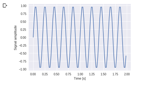
Vous pouvez le voir. La fréquence est de 5 Hz et son signal se répète en 1/5 seconde - c'est un appel pendant une période de temps particulière.
Utilisons maintenant cette onde sinusoïdale à l'aide de l'application DFT.
from scipy import fftpack

A = fftpack.fft(a)
frequency = fftpack.fftfreq(len(a)) * fre_samp
figure, axis = plt.subplots()

axis.stem(frequency, np.abs(A))
axis.set_xlabel('Frequency in Hz')
axis.set_ylabel('Frequency Spectrum Magnitude')
axis.set_xlim(-fre_samp / 2, fre_samp/ 2)
axis.set_ylim(-5, 110)
plt.show()
Sortie :
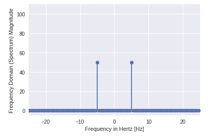
- Vous pouvez clairement voir que la sortie est un tableau unidimensionnel.
- Les entrées contenant des valeurs complexes sont zéro sauf deux points.
- Dans l'exemple DFT, nous visualisons l'amplitude du signal.
Optimisation et ajustement dans SciPy - scipy.optimize
- L'optimisation fournit un algorithme utile pour minimiser l'ajustement de courbe, multidimensionnel ou scalaire et l'ajustement de racine.
- Prenons un exemple de une fonction scalaire, pour trouver la fonction scalaire minimale.
%matplotlib inline
import matplotlib.pyplot as plt
from scipy import optimize
import numpy as np

def function(a):
       return   a*2 + 20 * np.sin(a)
plt.plot(a, function(a))
plt.show()
#use BFGS algorithm for optimization
optimize.fmin_bfgs(function, 0)
Sortie :
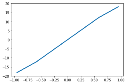
L'optimisation s'est terminée avec succès.
Valeur actuelle de la fonction :-23,241676
Itérations :4
Évaluations de fonction :18
Évaluations de dégradé :6
tableau([-1.67096375])
- Dans cet exemple, l'optimisation est effectuée à l'aide de l'algorithme de descente de gradient à partir du point initial
- Mais le problème possible est les minima locaux au lieu des minima globaux. Si nous ne trouvons pas de voisin des minima globaux, nous devons appliquer une optimisation globale et trouver la fonction de minima globaux utilisée comme basinhopping() qui combine l'optimiseur local.
optimiser.basinhopping(fonction, 0)
Sortie :
fun: -23.241676238045315
 lowest_optimization_result:
      fun: -23.241676238045315
 hess_inv: array([[0.05023331]])
      jac: array([4.76837158e-07])
  message: 'Optimization terminated successfully.'
     nfev: 15
      nit: 3
     njev: 5
   status: 0
  success: True
        x: array([-1.67096375])
                    message: ['requested number of basinhopping iterations completed successfully']
      minimization_failures: 0
                       nfev: 1530
                        nit: 100
                       njev: 510
               x: array([-1.67096375])
Algorithme Nelder-Mead :
- L'algorithme de Nelder-Mead sélectionne via le paramètre de méthode.
- Il fournit le moyen le plus simple de minimisation pour une fonction de comportement équitable.
- L'algorithme de Nelder – Mead n'est pas utilisé pour les évaluations de gradient, car la recherche de la solution peut prendre plus de temps.
import numpy as np
from scipy.optimize import minimize
#define function f(x)
def f(x):
    return .4*(1 - x[0])**2

optimize.minimize(f, [2, -1], method="Nelder-Mead")
Sortie :
final_simplex: (array([[ 1.        , -1.27109375],
       [ 1.        , -1.27118835],
       [ 1.        , -1.27113762]]), array([0., 0., 0.]))
           fun: 0.0
       message: 'Optimization terminated successfully.'
          nfev: 147
           nit: 69
        status: 0
       success: True
             x: array([ 1.        , -1.27109375])
Traitement d'images avec SciPy - scipy.ndimage
- scipy.ndimage est un sous-module de SciPy qui est principalement utilisé pour effectuer une opération liée à l'image
- ndimage désigne l'image à "n" dimensions.
- SciPy Image Processing fournit la transformation géométrique (rotation, recadrage, retournement), le filtrage d'image (net et débroussaillage), l'image d'affichage, la segmentation d'image, la classification et l'extraction de caractéristiques.
- Forfait MISC dans SciPy contient des images prédéfinies qui peuvent être utilisées pour effectuer une tâche de manipulation d'images
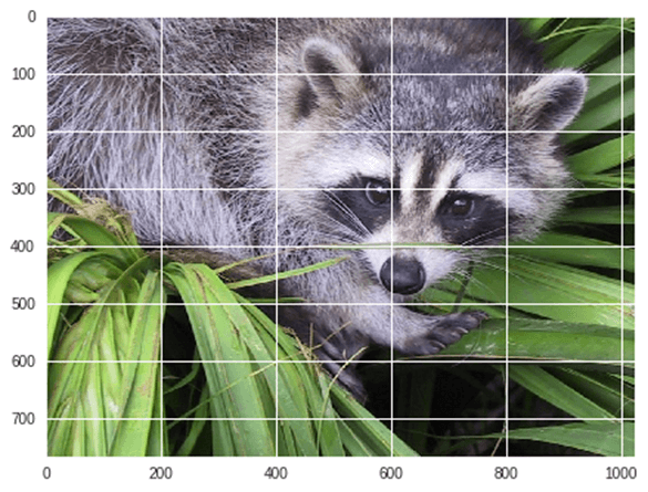
Exemple : Prenons un exemple de transformation géométrique d'images
from scipy import misc
from matplotlib import pyplot as plt
import numpy as np
#get face image of panda from misc package
panda = misc.face()
#plot or show image of face
plt.imshow( panda )
plt.show()
Sortie :

Maintenant, nous Replions image actuelle :
#Flip Down using scipy misc.face image
flip_down = np.flipud(misc.face())
plt.imshow(flip_down)
plt.show()
Sortie :
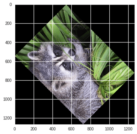
Exemple : Rotation de l'image à l'aide de Scipy,
from scipy import ndimage, misc
from matplotlib import pyplot as plt
panda = misc.face()
#rotatation function of scipy for image – image rotated 135 degree
panda_rotate = ndimage.rotate(panda, 135)
plt.imshow(panda_rotate)
plt.show()
Sortie :
Intégration avec Scipy - Intégration numérique
- Lorsque nous intégrons une fonction où l'intégration analytique n'est pas possible, nous devons nous tourner vers l'intégration numérique
- SciPy fournit des fonctionnalités pour intégrer la fonction avec l'intégration numérique.
- scipy.integrate bibliothèque a une intégration simple, double, triple, multiple, quadrate gaussien, règles de Romberg, trapézoïdales et de Simpson.
Exemple : Prenons maintenant un exemple d'intégration unique

Ici un est la limite supérieure et b est la limite inférieure
from scipy import integrate
# take f(x) function as f
f = lambda x : x**2
#single integration with a = 0 & b = 1
integration = integrate.quad(f, 0 , 1)
print(integration)
Sortie :
(0.3333333333333337, 3.700743415417189e-15)
Ici, la fonction renvoie deux valeurs, dans lesquelles la première valeur est l'intégration et la seconde valeur est l'erreur estimée dans l'intégrale.
Exemple :Prenons maintenant un exemple SciPy de double intégration. On trouve la double intégration de l'équation suivante,
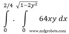
from scipy import integrate
import numpy as np
#import square root function from math lib
from math import sqrt
# set  fuction f(x)
f = lambda x, y : 64 *x*y
# lower limit of second integral
p = lambda x : 0
# upper limit of first integral
q = lambda y : sqrt(1 - 2*y**2)
# perform double integration
integration = integrate.dblquad(f , 0 , 2/4,  p, q)
print(integration)
Sortie :
(3.0, 9.657432734515774e-14)
Vous avez vu cette sortie ci-dessus comme la même précédente.
Résumé
- SciPy (prononcez "Sigh Pi") est une bibliothèque Open Source basée sur Python, qui est utilisée dans les mathématiques, le calcul scientifique, l'ingénierie et le calcul technique.
- SciPy contient une variété de sous-paquets qui aident à résoudre le problème le plus courant lié au calcul scientifique.
- SciPy est intégré au-dessus de NumPy
| Nom du package | Description |
|---|---|
| scipy.io |
|
| scipy.special |
|
| scipy.linalg |
|
| scipy.interpoler |
|
| scipy.optimize |
|
| scipy.stats |
|
| scipy.integrate |
|
| scipy.fftpack |
|
| scipy.signal |
|
| scipy.ndimage |
|
Python
- Instruction Python Print() :comment imprimer avec des exemples
- Python String count() avec des EXEMPLES
- Fonctions Python Lambda avec EXEMPLES
- Fonction Python abs() :Exemples de valeurs absolues
- Fonction Python round() avec EXEMPLES
- Fonction Python map() avec EXEMPLES
- Python Timeit() avec des exemples
- Rendement en Python Tutoriel :Exemple de générateur et rendement vs retour
- type() et isinstance() en Python avec des exemples